Auto-Labeling Images with CLIP and K-Means

Motivation

In practice, there are many cases that require human effort to review unknown images for mismatched labeling, flagging anomalies, and verifying policy compliance. Manually labeling thousands of images takes a lot of effort, and it is exhausting. What if there is a way to simplify this process? Instead of running through each image to assign a label, we could reduce the workload by just reviewing some samples, and the system will automatically assign similar images with the same label.

CLIP, a multimodal model that embeds both images and texts, solves this. Its embedding space organizes images in a semantic order where a photo of a dog is close to animals like cats and sheep but far from vehicles like bikes and cars.

You can follow along with the complete implementation in the Kaggle Notebook.

Note: I’m currently updating the Kaggle notebook to run smoothly with CUDA. The original code was developed and run on my MacBook (MPS), so the Kaggle version is still a work in progress.

Pipeline Overview

1. Encoding: CLIP encodes images and L2-normalizes them into a 512D embedding space.
2. Visualization: plot UMAP 2D to visually inspect K, the number of clusters.
3. Clustering: find optimal dimension D for PCA, L2-normalize, and apply K-means.
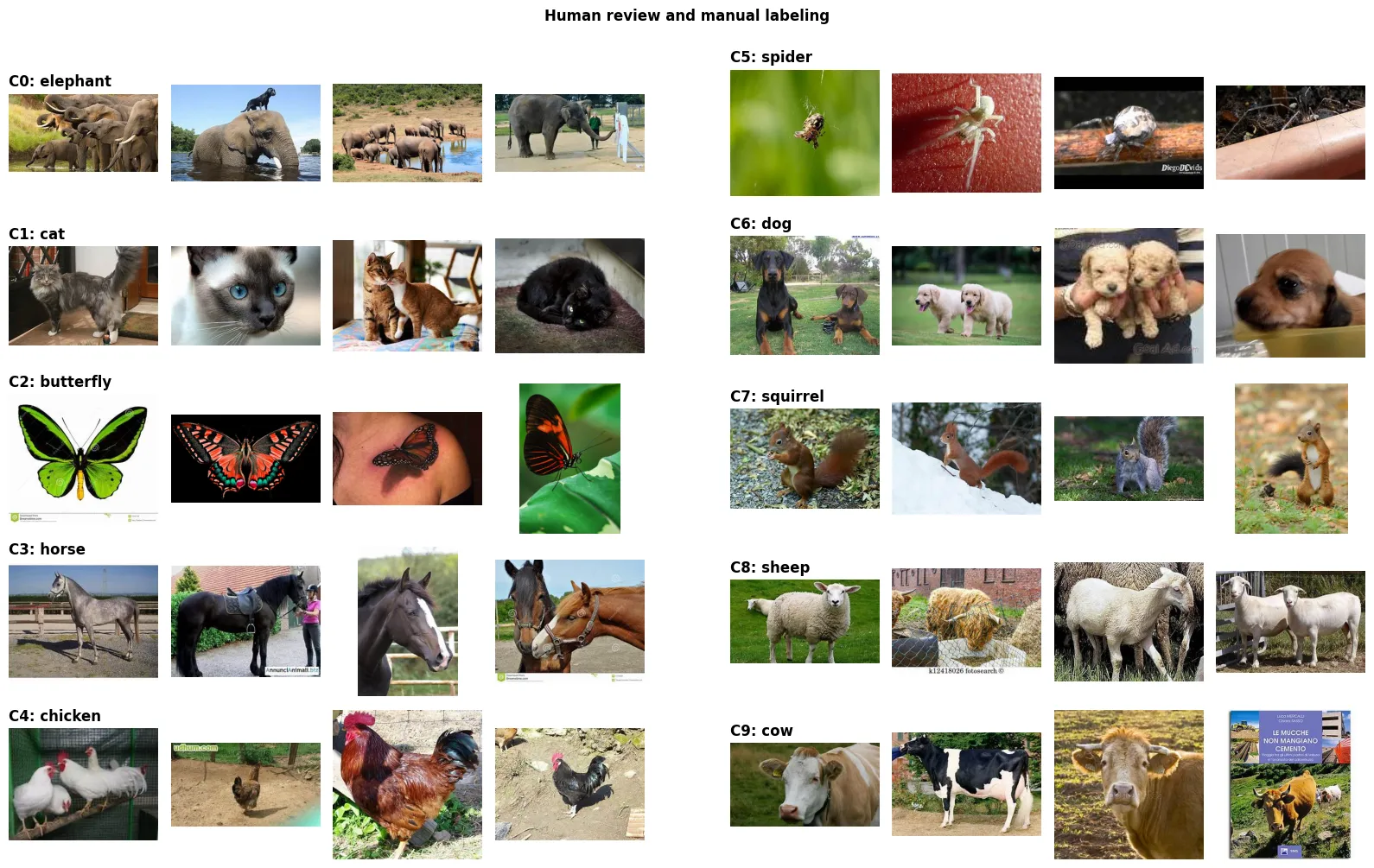
4. Labeling: reviewing 3~4 images from each cluster and naming the cluster.
5. Saving: PCA + centroids + labels for reusing to classify unseen images in the future.

Dataset

We use the Animals-10 dataset from Kaggle to demonstrate the concept. It contains 26,179 images; the classes of animals have an imbalanced distribution. The dataset contains 10 animals with labels in Italian, but we flatten them into one single array for clustering.

Before continuing, we split 500 images from the dataset to hold out and process only the 25,679 images. We will use the hold-out set for evaluation in a later article.

1
Full dataset (26,179 images)
2
├── Hold-out (500)        → FROZEN for upcoming articles
3
└── Working pool (25,679) → available in this article

UMAP 2D Visualization

The power of UMAP is that it can capture nonlinear structures and visualize data from a 512-dimensional embedding space on a 2D scatter, making it possible for people to visually examine and investigate the data’s hidden patterns.

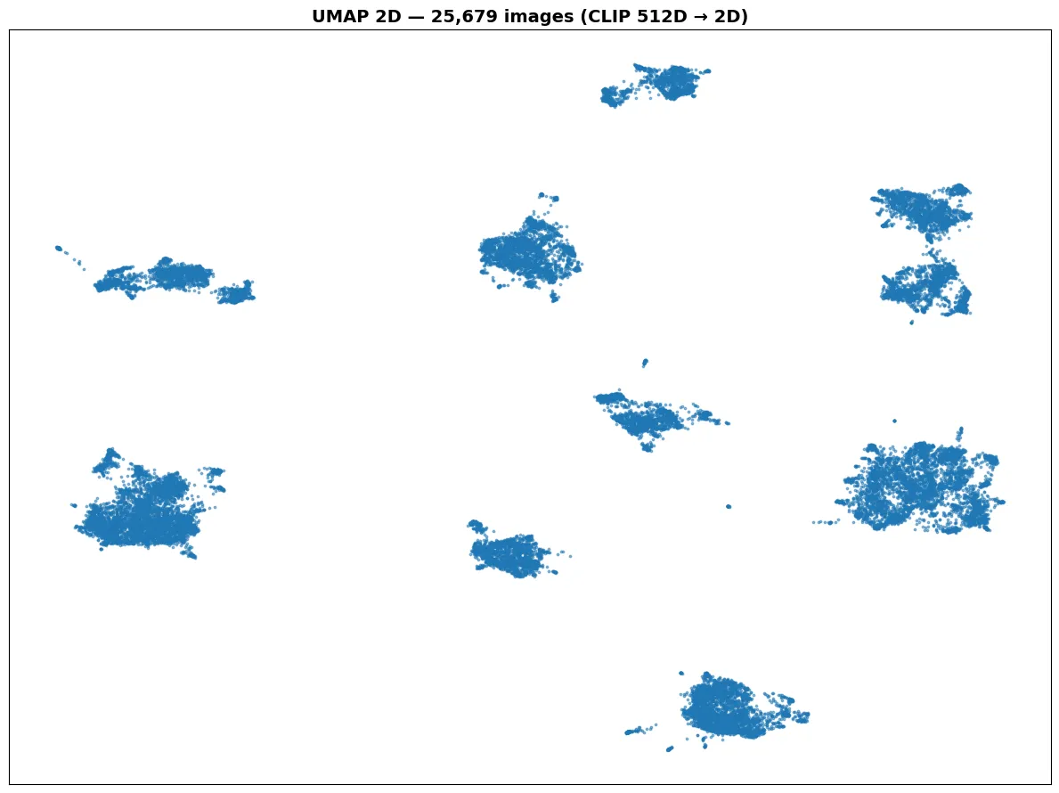
Based on the plot, we can see that 10 distinct groups are cleanly separated; the only confusion is the top-right has 2 clusters with a thin link that may confuse us.

We use UMAP as an exploratory step to get a rough estimation of K. Running the silhouette score directly in 512D could give misleading results. K-Means is Euclidean distance-based; using it in high-dimensional space produces unreliable results due to the curse of dimensionality, where everything has the same distance from a point.

K-Means on 512D

Now, let’s see if we run K-means directly on the 512D dataset. It’s surprising that the best K is 10, which is determined by the highest silhouette score 0.180.

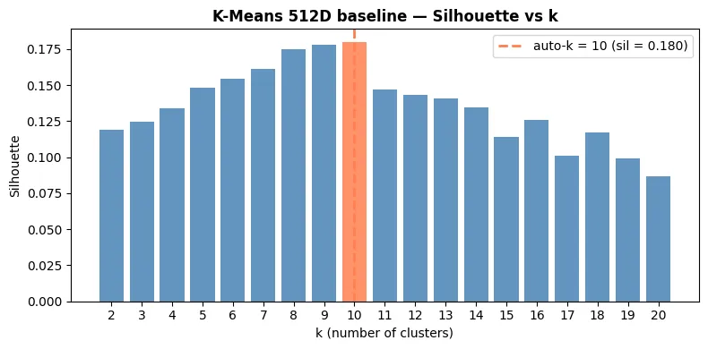
However, it’s a very low score, which indicated that the clustering algorithm failed to create well-separated groups. To increase the silhouette score, we can apply PCA to reduce the curse of dimensionality, but what dimension should we reduce? What if we consider D as a hyperparameter?

PCA with D as a Hyperparameter

PCA filters noises and reduces the curse of dimensionality to restore the accuracy of clustering-based metrics like Euclidean distance in low dimensions.

To find the optimal D, we sweep through 8, 12, 16, and so on to 128 to find the best D that can achieve the highest silhouette score with K = 10 clusters.

Note: We set K = 10 because our earlier visual inspection via UMAP showed that the data forms 10 distinct clusters.

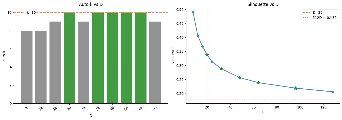
As a result, reducing 512D to 20D increases the silhouette score to 0.338 (improved +0.158), which improves the performance of the K-means clustering.

Clustering

This brings us to the final stage of the pipeline. With the optimal dimension of 20D, we run K-Means and find the clusters and their centroids.

Centroids are the key of the next post, where we can identify unseen images not in the original dataset, but for now our objective for this topic is achieved. We are able to identify the label for all the images.

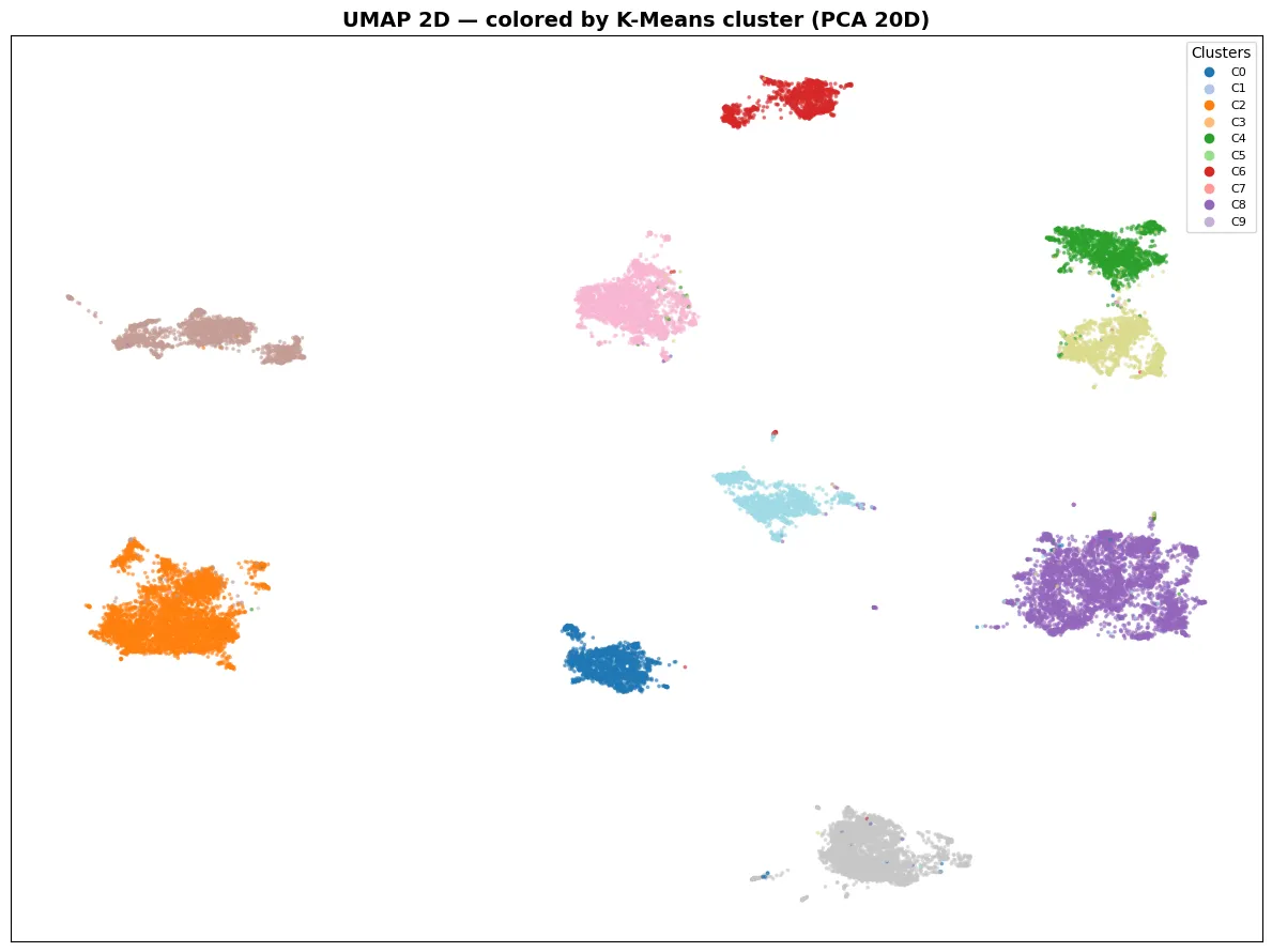
Let’s review by plotting UMAP with colors of identified clusters; it shows that K-means works well with what was discovered from the visual inspection.

Human Review

Instead of manually labeling 25,679 images, we only need to review 4 samples per cluster. Automated labeling successfully handled 99.8% of the dataset.

(25,679 - 40) ÷ 25,679 = 99.8% automated labeling coverage

Conclusion

In the future, when new images come in, the system can reuse these centroids to classify unseen images, which will be discussed in the next posts.

This demonstration project shows a combination of traditional machine learning with deep learning to solve image problems; if we apply it at scale, we can solve real-world problems.

The open question is what if the new photo is not of these classified animals? What if it is an image of a fish?

References

• Corrado, A. (2019). Animals-10 (Version 2). Kaggle.