

Introduction
In the previous post, Auto-Labeling Images with CLIP and K-Means, we constructed a pipeline to encode a pool of images, reduce dimensionality with PCA, cluster them with K-Means, and auto-label whole images in each cluster via manually labeling a few samples.
However, there are two remaining questions:
-
How do we classify new unseen images?
-
Since we already know 10 distinct labels, how does this classification compare to CLIP zero-shot?
In this post, we will build a pipeline to classify unseen images and address the out-of-distribution problem, specifically the question of how to classify an image of a fish in the pool of 10 animals. Then benchmark the accuracy of both approaches using the 500 hold-out images from the previous post.
You can follow along with the complete implementation in the Kaggle Notebook.
Dataset
We continue using the Animals-10 dataset from Kaggle, but in this article, we only use 500 holdout images for classification and evaluation.
Each group contains 50 images of 10 animals; we apply the same random seed to restore the holdout images from the previous post.
Holdout (500 images)├── 50 × dog├── 50 × cat├── 50 × horse├── 50 × chicken├── 50 × sheep├── 50 × cow├── 50 × spider├── 50 × butterfly├── 50 × elephant└── 50 × squirrelNearest Centroid Classification
Reusing Centroids
We reuse the saved centroids found from the clustering algorithm in the previous post to construct a pipeline to classify a new incoming unseen image.
- Encode the new image using CLIP and L2-normalize → 512D vector
- PCA reduces dimension using the saved PCA transformer and L2-normalize → 20D vector
- Calculate the cosine similarity between the projected point with all 10 centroids.
- Assign the label of the nearest centroid (highest similarity score) to the image.
Note: Because the centroids were constructed using K-Means in 20D space, we have to apply the same PCA transformation to the new incoming image before we can compare their similarities.
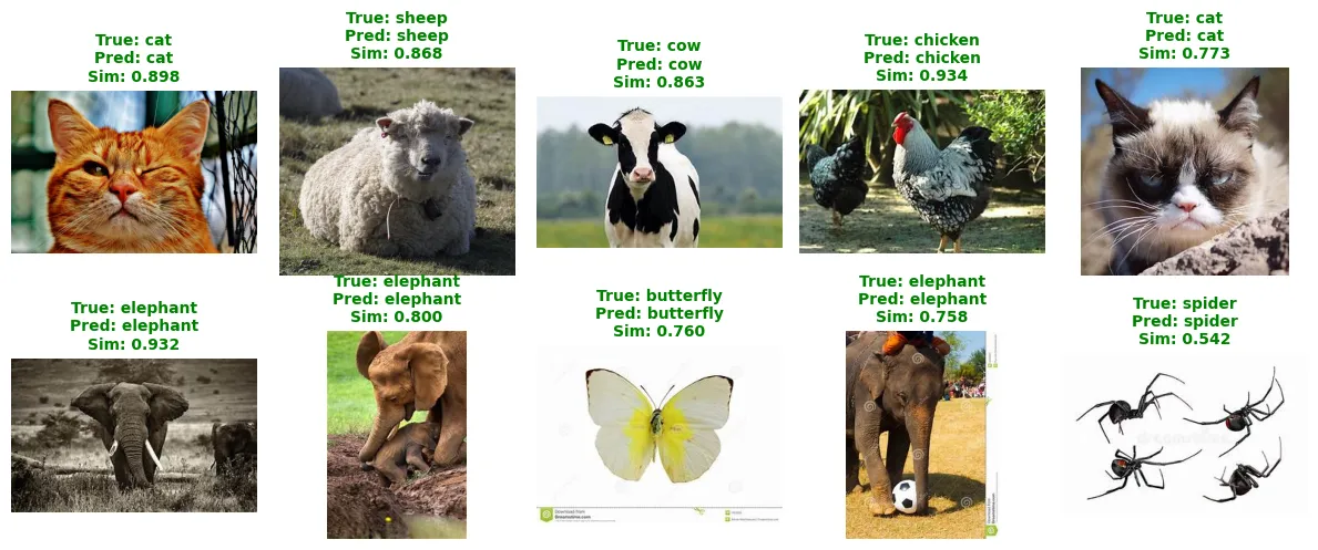
Classify Holdout Images
In this scenario, we already know the label of these animals, but we fit it into the classification pipeline to evaluate our algorithm.
The process involves scanning 500 images and computing the cosine similarity against the 10 centroids to find the closest one (highest similarity score). Then assign its label to the image.
Handling Out-of-Distribution
Confidence Threshold
The current pipeline has a problem when the input image does not belong to the 10 animals. What if a user uploads a fish image? It will run through 10 centroids to find the nearest one and then assign the label of that centroid to the image.
To resolve this problem, we set a threshold; if the cosine similarity to the nearest centroid is lower than the threshold, we classify the image as unknown. Then the out-of-distribution image will need a human to review.
In our 10-animals example, we calculate a dynamic threshold using the 25,679 images from the previous post. We set the 10th percentile of this score distribution as our threshold, which is 0.634; any input image with a similarity score lower than 0.634 will be flagged as unknown.
Note: We obtain this confidence threshold by calculating the cosine similarity between each of the 25,679 images with all 10 centroids.
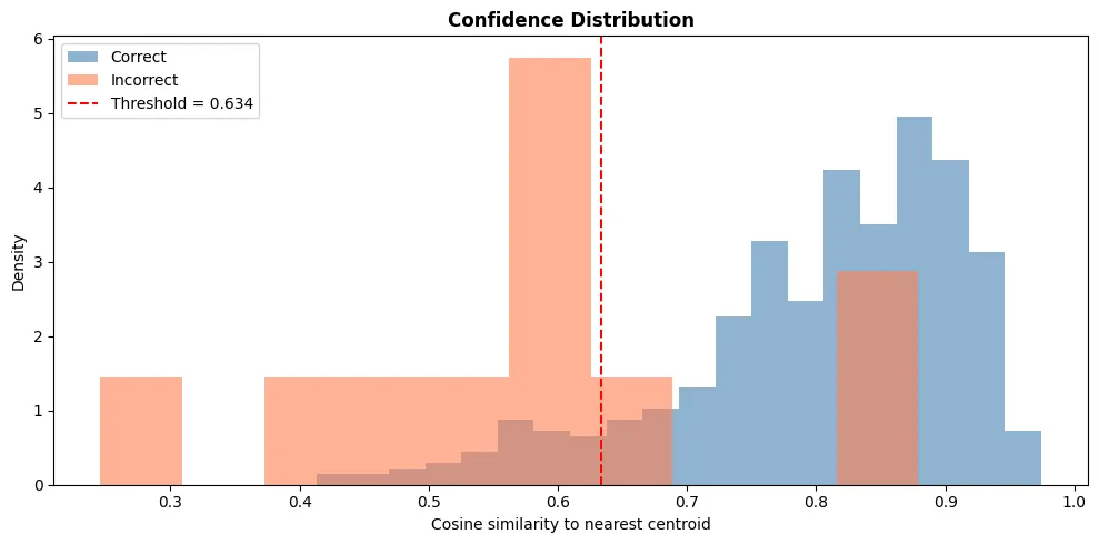
As introduced in the previous post, automated labeling successfully handled 99.8% of the dataset. When we apply a similarity threshold, automated labeling still covers 89.0% of the holdout dataset, leaving the remaining 11% (55 images) flagged for manual verification.
Testing the threshold with a fish image
This is a photo that I took to simulate the user uploading an abnormal image into the classification system.
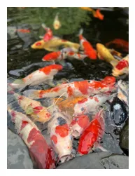
Surprisingly, it is assigned to the butterfly centroid with a similarity score of 0.488, but with the introduced threshold, it will be marked as unknown, flagging it as an anomaly that does not match known patterns.
This finally establishes a complete classification pipeline.
- Encode the new image using CLIP and L2-normalize → 512D vector
- PCA reduces dimension using the saved PCA transformer and L2-normalize → 20D vector
- Calculate the cosine similarity between the projected point with all 10 centroids.
- Compare the similarity score with the threshold; if it’s lower than the threshold, flag it as unknown.
- Otherwise, assign the label of the nearest centroid (highest similarity score) to the image.
Images Flagged in the Holdout dataset
Let’s run again the 500 images, but this time with a threshold of 10% to flag for human review.
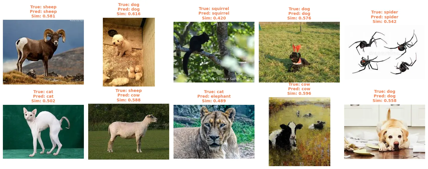
For example, we found an image of a tiger that was mislabeled as a “cat” in the original dataset. Our system matched it to the “elephant” centroid, but because the prediction confidence was extremely low, the score dropped below our threshold. As a result, the system successfully flagged this image for human review instead of incorrectly labeling it. This proves our safety threshold successfully catches noisy ground-truth data.
Through this flag, we successfully detected a noisy ground-truth anomaly (a tiger image placed in the cat dataset). In the next post, we will explore how to detect such anomaly images within our training pool.
CLIP Zero-Shot Classification
We already know the 10 species names, instead of running through our centroids with a threshold, we can directly run it with CLIP zero-shot classification. It is simple; we just define 10 text prompts for our classes.
- “a photo of a dog”
- “a photo of a cat”
We then compare the cosine similarity between the image embedding and the text embeddings of these prompts to assign the label.
With the given 500-image dataset, it gives us 98% accuracy of this example.
But why not use CLIP Zero-Shot in the first place? A major advantage of our centroid pipeline is that it is completely vocabulary-free.
It does not depend on crafting the perfect text prompt or knowing the domain knowledge. Instead, the visual features group naturally, and we can simply assign a label to the cluster.
Evaluation
In this balance across all classes, we use the accuracy metric to evaluate the model.
Total images: 500
| Method | Correct | Mismatches | Accuracy | Needs Manual Review |
|---|---|---|---|---|
| Without threshold | 489 | 11 | 97.8% | 0 |
| With 10% threshold | 442 | 3 | 99.3% | 55 |
| CLIP Zero-Shot | 490 | 10 | 98.0% | 0 |
Note: The threshold accuracy of 99.3% is measured only over 89.0% (445 images), the remaining 11% require a human to review.
Conclusion
This post demonstrates the efficiency of classifying unknown images and detecting anomalies using clustering centroids. This approach can be easily scaled to real-world use cases:
- Mismatched labeling: Find mistakes made by human annotators (e.g., the tiger labeled as a cat found in the Animals-10 dataset).
- Dataset cleaning: We use this exact approach to automatically identify and remove anomalies, cleaning public datasets before we use them for training.
- Fraud detection foundation: Provides a baseline signal to flag uploaded images that do not match any known cluster or pattern. Turning this into a real fraud detector would additionally require domain-specific logic, risk heuristics, and a dedicated classifier.
However, this centroid-based approach is not the optimal way to detect anomalies or find suspicious images hidden inside a dataset. In the next post, we will apply Isolation Forest to truly hunt down anomalies and suspicious images inside the 10-Animals dataset.
References
- Corrado, A. (2019). Animals-10 (Version 2). Kaggle.
- Nguyen, J. (2026). Classifying Images with K-Means Centroids. Kaggle.