

Introduction
While working with the Animals-10 dataset in the previous post about classifying images with K-Means, I found that the dataset is quite messy and unclean. But thanks to that mess, I tried a method to find anomalous images in the dataset. It is like finding the “impostors” in Among Us, where the tiger images are hidden in the cat category.
Having noise in the model training process is likely to degrade model performance, especially with image datasets. It wastes computing resources if we input low-quality images to the training. In this article, I want to introduce a combined tree decisions method using Isolation Forest to efficiently spot anomalous images, leveraging the semantic understanding of image content from CLIP embeddings.
See the full code and results here: Detecting Anomalies with Isolation Forest on CLIP (Kaggle).
Dataset
We continue using the Animals-10 dataset from Kaggle to experience the anomaly detection pipeline. The dataset contains 26,179 images of 10 different species with an imbalanced distribution.
To find anomalies in each class, we keep the original structure of the dataset to process independently in each class.
The Workflow
Our workflow looks like this:
- Feature Extraction: Convert all 26,179 images into 512-dimensional CLIP embeddings.
- PCA Sweep: Iterate through dimensions [128, 64, 32, 16].
- Per-Class Isolation: Run an Isolation Forest for every species at every dimension.
- Intersection: Identify the “overlapping anomalies” that are flagged in every single PCA dimension.
The Core Algorithm
Feature Extraction with CLIP
When working with tabular data, we have to deal with feature engineering types: numerical and categorical columns, but OpenAI CLIP offers feature extraction for free when processing the images.
By using the model ViT-B/32, each image is embedded in a space with 512 dimensions, which are considered 512 features to distinguish between images and are ready to be input into the anomaly algorithm without any manual processing.
Understanding Isolation Forests
To visually demonstrate the concept of Isolation Forest, we create a toy dataset that contains 10 images:
- 9 images of cats
- 1 image of a tiger playing the role of an impostor among the cats
See the notebook for this example here: The Tiger: An Imposter Among Cats (Kaggle).
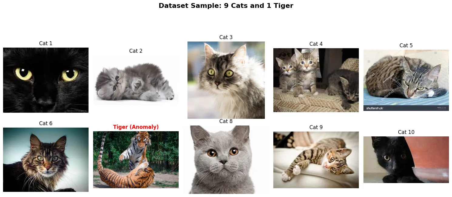
Sample dataset with random distribution for the algorithm to find the tiger.
Reducing to Two Features
The CLIP embeddings have 512 dimensions, which means we cannot visualize and inspect the splits of the algorithm on a scatterplot. Therefore, we apply the PCA method to reduce 512D to 2D, which we can think of as 2 features, PC1 and PC2, so we can plot the 10 images on the graph. It enables us to visually follow the process to isolate the tiger in the next few steps.
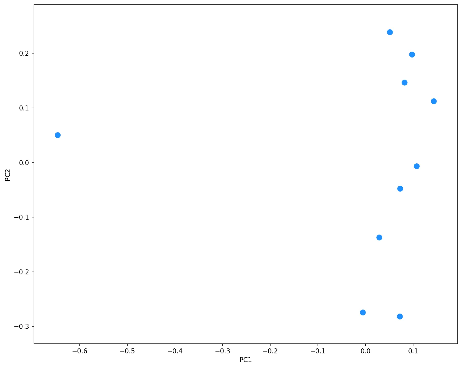
A 2D PCA projection reveals a clear outlier in the dataset.
The Isolation Tree
An isolation tree is essentially a binary search tree. Instead of finding a value, it recursively splits the data randomly in the following steps:
- Pick a random feature. In the original 512D, it randomly picks from 1 to 512 features, but we have simplified it into 2 features. In this example, it picks randomly between PC1 and PC2.
- In the selected feature, find the min and max values and make a random split between them.
- The split divides the partition into 2 nodes.
- Repeat this recursively until each node meets a stop condition:
- Each leaf node has only one instance.
- A predefined maximum depth is reached.
The idea is simple: each outlier will be found at the leaf nodes with the shortest path to the root. This is because the outlier is far from dense nodes, so it will be isolated quickly. In contrast, normal points are located in dense areas, which will need more continuous splits to reach the leaf node, and the traverse path is longer.

The splitting process in BST format:
- 1st slice (root): It contains 10 images. The first split randomly picks PC2 and makes a horizontal cut, dividing the root node into 2 child nodes: the left node contains 6 images, and the right node contains 4 images.
- 2nd slice (left recursive - 6 images): This group continuously divides into 2 partitions by randomly splitting PC1. This slice immediately isolates the leaf node. The stop condition has been met, and the tiger image is isolated just after 2 splits from the root.
- The other slices (recursive from other nodes): Cat images are grouped together; it likely requires more than 3 to 4 splits until the stop condition.
The traversal path of the tiger after 2 splits is shorter than the path of any cat in the current tree. This is proof that the tiger image is an outlier in the binary search tree.
From Tree to Forest
A single tree depends on its random splits, meaning any single model may come with bias. Because it is random, a tree may accidentally isolate a normal point, like an innocent cat in just a few splits.
Instead of asking a tree for an opinion, why don’t we ask more trees to aggregate their opinions with different biases? Finally, we average their opinions to make a final decision. The one that is always quickly isolated in a crowd with different biases will likely be the anomaly point.
To have a visual, we create 5 trees to simulate the experiment.
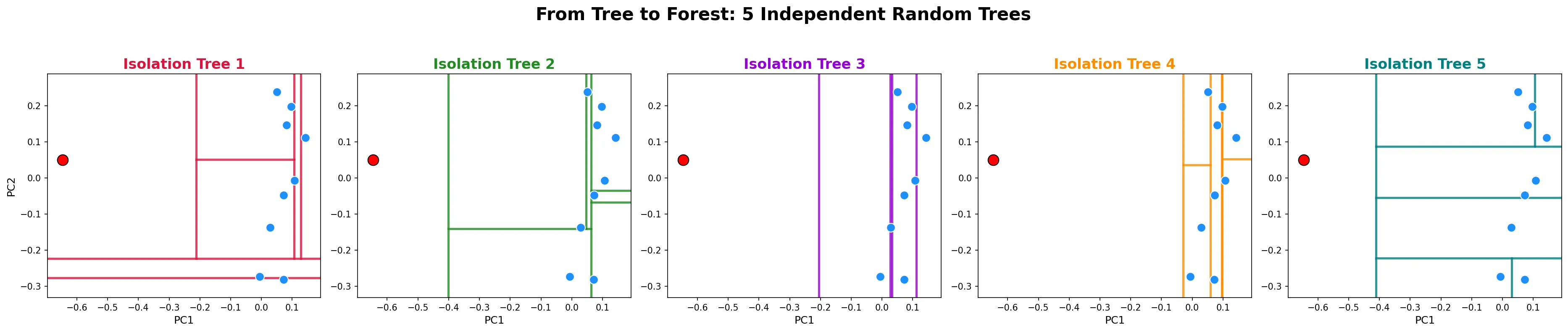
Splits to isolate the tiger (red dot) in 5 independent trees:
| Tree 1 | Tree 2 | Tree 3 | Tree 4 | Tree 5 |
|---|---|---|---|---|
| h = 2 | h = 1 | h = 1 | h = 2 | h = 1 |
Now with the opinion h from 5 trees, how do we aggregate them into one decision? The answer is to average and normalize into an anomaly score.
The anomaly score of each point is calculated based on the average depth from all the trees in the forest:
| Symbol | Meaning |
|---|---|
| h(x) | Depth of point x in a single tree |
| E(h(x)) | Average of h(x) across the entire forest - aggregating all opinions from the trees |
Where is the normalization constant - the theoretical average depth of a BST with n samples, and is the Euler-Mascheroni constant ≈ 0.5772:
Applying this to our small dataset with n=10, we plug the numbers into c(n):
The average depth of the tiger across 5 trees is E(h) = (2+1+1+2+1)/5 = 1.40, which means:
To clearly see how the tiger stands out compared to the cats, here are the scores for all 10 images:
| Image | E(h) | s | Image | E(h) | s | |
|---|---|---|---|---|---|---|
| Cat 1 | 3.20 | 0.4969 | Cat 6 | 3.20 | 0.4969 | |
| Cat 2 | 4.00 | 0.4172 | Cat 7 | 3.80 | 0.4358 | |
| Cat 3 | 3.20 | 0.4969 | Cat 8 | 4.00 | 0.4172 | |
| Cat 4 | 3.60 | 0.4553 | Cat 9 | 3.60 | 0.4553 | |
| Cat 5 | 4.00 | 0.4172 | Tiger | 1.40 | 0.7384 |
The tiger has a score of 0.7384 - the highest and clearly separated from all 9 cats (0.41–0.49). Based on the score reading table below, this proves that the tiger is an anomaly:
| Score s | Meaning | Decision |
|---|---|---|
| s ≈ 1 | Isolated very quickly in most of the trees | Anomaly |
| s ≪ 0.5 | Needs many splits to be separated | Normal |
| s ≈ 0.5 in total | No point stands out | No clear anomaly |
Scaling to Full Dataset
Reducing Dimensions
When I tried the algorithm on the raw 512D, the results were not good. It was hard to detect the anomalies; most were false positives. Then I tried to reduce the dimension to 128D; the results were better. Checking the outlier images, I could see out-of-distribution images within the class, but what is the optimal dimension to reduce to? If we cannot find one target dimension, then we sweep through multiple dimensions and finally take the intersection of the results. For example, I chose dimensions from 128, 64, 32, and 16; ran each separately; and then took only the overlap-flagged images.
Contamination Thresholds
The current workflow uses IsolationForest from scikit-learn with a contamination threshold, meaning if we set contamination=0.01, the algorithm is forced to find 1% anomalies in the dataset. However, in this scenario, we don’t know how many outlier images are in the dataset; the better way is just to set it to auto and leave the decision to the algorithm.
Running a multi-dimensional sweep with the Animals-10 dataset, the algorithm found exactly 231 overlapping anomalies from 26,179 images, about 0.88% of the distribution.
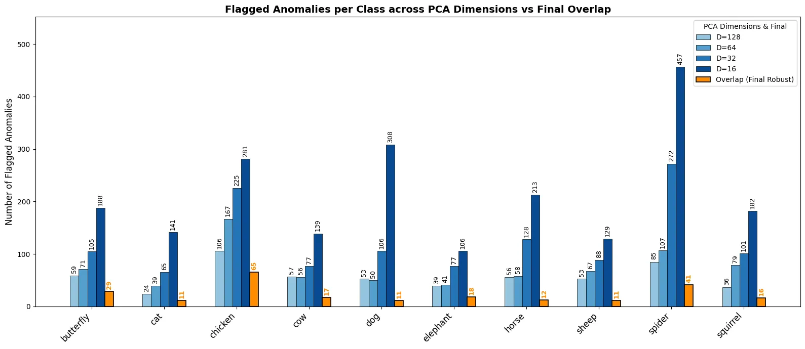
In lower dimensions, Isolation Forest seems to find more anomalies than in high-dimensional ones. Similar to asking multiple trees in the forest, now it’s like asking for results from multiple dimensions (the orange column).
Below is a detailed breakdown of the overlapping anomalies flagged for each class:
| Class | Total Images (N) | Flagged Anomalies | Anomaly Rate | True Anomalies | Precision |
|---|---|---|---|---|---|
| chicken | 3,098 | 65 | 2.1% | 26 | 40.0% |
| butterfly | 2,112 | 29 | 1.4% | 28 | 96.5% |
| elephant | 1,446 | 18 | 1.2% | 6 | 33.3% |
| cow | 1,866 | 17 | 0.9% | 7 | 41.2% |
| squirrel | 1,862 | 16 | 0.9% | 3 | 18.8% |
| spider | 4,821 | 41 | 0.9% | 23 | 56.1% |
| cat | 1,668 | 11 | 0.7% | 10 | 90.9% |
| sheep | 1,820 | 11 | 0.6% | 5 | 45.5% |
| horse | 2,623 | 12 | 0.5% | 2 | 16.7% |
| dog | 4,863 | 11 | 0.2% | 8 | 72.7% |
| Global | 26,179 | 231 | 0.88% | 118 | 51.1% |
After manually reviewing all 231 flagged images, I found that 118 of them were true out-of-distribution anomalies; the remaining are low-quality images but acceptable, giving a global precision of 51.1%. Not a perfect score, but a massive time-saver.
Note: We cannot calculate an exact recall for this experiment because the dataset lacks ground-truth labels. However, assuming the vast majority of the 26,179 images are correctly labeled and there are very few true anomalies in total, the recall for this pipeline is likely very high.
Visualizing Within-Class Anomalies
Now let’s see the flagged images from the algorithm. By sorting the anomaly scores in ascending order among the flagged items, we get the most extreme outliers in each class.

In the Cat class, the algorithm clearly spots tigers, paintings, trees, and mountains with no animals. By reducing the dimensions, the lower dimensions gain more signal to find the different context between the images and boost the Isolation Forest to spot these outliers.
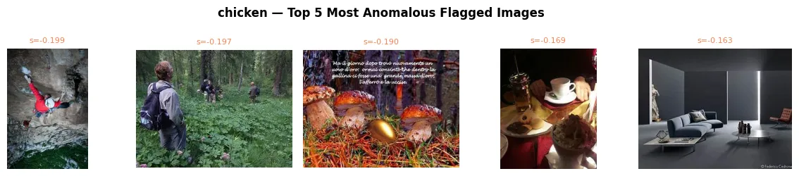
Similarly, in the Chicken class, our workflow isolated images of people, mushrooms, paintings, and house decorations mixed into the chicken category.
Because the dataset contains a significant amount of noisy, weird, and sometimes inappropriate images scraped from the web, we have limited the visual examples here. To see the full top 20 global anomalies and explore the entire pipeline, check out the full notebook on Kaggle!
UMAP 2D Visual Projection
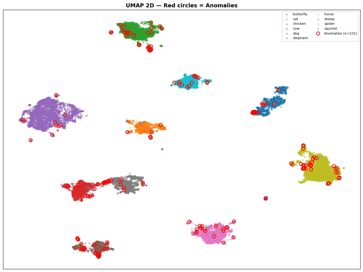
To get a big picture of where anomalies are distributed in each class, we use UMAP to project the 512D embeddings into a 2D scatterplot. It helps to show the dense clusters of each animal in the dataset, and the red circles are anomalies located near the border of each cluster.
Use Cases & Limitations
This methodology demonstrates a proof-of-concept for filtering noisy images, but it still needs a human in the loop. How you use it depends on the strictness of the work. For my example, I could easily accept clearing all 231 flagged images, false positives included. In a stricter setting, ~50% precision still saves real time: instead of manually reviewing 26,179 images, you only check 231.
Furthermore, the model we use is the weakest CLIP model (ViT-B/32) for POC convenience, meaning its performance with larger models (ViT-L/14) on complex real-world datasets remains untested.
Conclusion
Why not just prompt “a photo of a tiger” to find the tiger in the cat category? It is because we don’t even know what outlier content is hidden inside the dataset. Isolation Forest resolves this problem by systematically identifying anomaly points in the semantic embedding space where we don’t have to input any domain knowledge, demonstrating the power of unsupervised learning.
References
- Corrado, A. (2019). Animals-10 (Version 2). Kaggle.
- DataCamp. Isolation Forest in Python.
- Nguyen, J. (2026). Detecting Anomalies with Isolation Forest on CLIP. Kaggle.
- Nguyen, J. (2026). The Tiger: An Imposter Among Cats. Kaggle.